Raster Analysis with QGIS
If you are new to rasters, check out our first part of the raster series about what rasters are in here.
As stated in the previous blog post, rasters are usually a bit harder to manage than vectors. There are different types of rasters you could use: there are different aerial images (satellite, plane, drone etc.), surface models for example digital elevation models (DEM) or digital surface models (DSM) that tell the elevation of the pixel above sea level. Or you could use just a plain old image taken with any camera.
In this example I downloaded 11 digital elevation models (DEM) from Paituli which is a download service that provides data from for example National Land Survey of Finland, University of Helsinki and Finnish Meteorological Institute. These elevation models are from the National Land Survey and they are in 2 x 2 m scale. This means that the pixel size in these models is 2m x 2m.
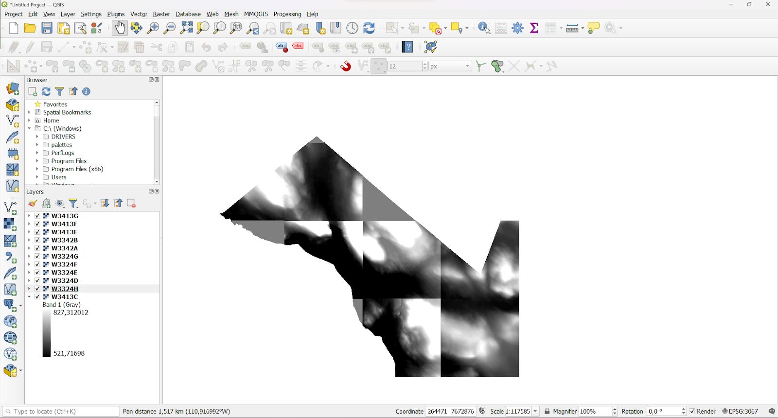
DEM tells the elevation of the area above the mean sea level. In these only bare ground is represented. In DSM all the objects on the surface of Earth, trees and buildings, are represented.
Merging rasters
In Finland surface models usually come in some kind of grid. Newer models are usually in TM35 map sheet division that is based on ETRS-TM35FIN coordinate reference system. Older ones before 2007 are in map division that is based on the KKS coordinate reference system. If you need to view a bigger area than just the one map sheet, you can merge the DEMs together very easily in QGIS!
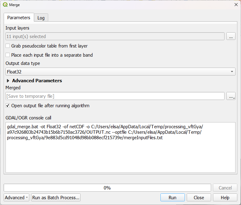
Open Raster -> Miscellaneous -> Merge. In the new window select all your individual rasters as input and run the algorithm.
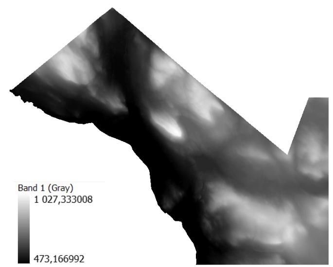
As a result you get one raster with the highest and the lowest elevation values in one like this:
Visualising the raster
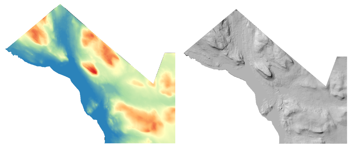
In the merged raster layer the highest point is the top of the Saana fjeld and the lowest is the lake Kilpisjärvi. To see the elevation distribution a bit better let’s change the visualisation. From layer properties change the symbology to Singleband pseudocolor. Here you can edit the colours and classify values for the visualisation. Hillshade is also a great option, if you want to view the elevation in different areas.
QGIS tools for rasters
Aside from visualisation techniques QGIS offers a wide range of algorithms to analyse your dataset. These can be found from the raster menu or from the Processing toolbox. The latter might offer a bit more tools. Let’s take a look at a few of the algorithms and why to use them!
Firstly hillshade. I know, I know this is also a visualisation technique but I promise this one looks way better. If you are looking closely at the visualisation hillshade it makes these small squares that are seen quite easily (the left picture below) as opposed to the hillshade made with the algorithm that is a better quality and looks way better zoomed in.
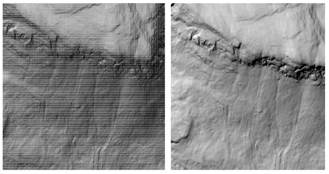
If you want to make a nice looking map, move the original visualised DEM on top of your newly calculated hillshade layer, change the symbology back to singleband pseudocolor and set the transparency to 40 %.
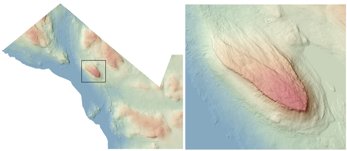
In hillshade you can change the azimuth and vertical angle of the sun. For example if you need to see how the terrain looks when the sun is shining from east at 90 degrees, this is where you can experiment. More on calculating hillshade in the QGIS documentation.
Some other algorithms that might prove to be useful when analysing terrain or for example trying to find a suitable place for a new wilderness hut could be slope and aspect.
Slope calculates the steepness of the terrain. For the wilderness hut you would need a relatively flat ground. The whiter the pixel, the steeper the terrain. Here are examples from Saana fjeld on the left and Ailakkavaara fjeld on the right.
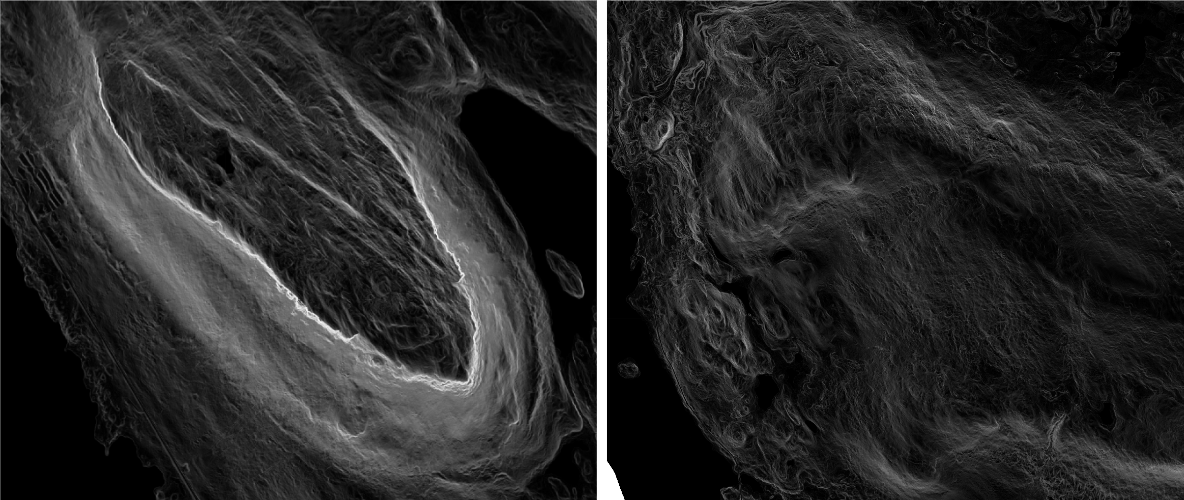
With a quick glance it would seem that Ailakkavaara could be more suitable for our wilderness hut. The last thing to consider is what kind of view our hut could have. With the aspect algorithm you can calculate the compass direction of your slopes.
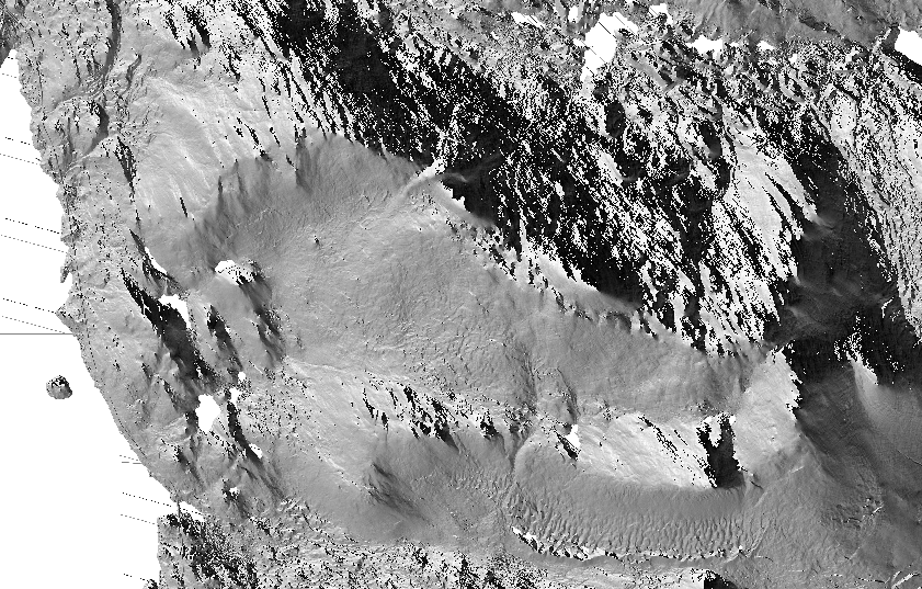
Here is a snippet of the data from Ailakkavaara fjeld. Let’s say we would want a north facing slope next to our hut to see the Saana fjeld when you get up in the morning. Here when the aspect is 0 the slope faces north. If 90 degrees the slope faces east etc. Seems that there are a few different potential places for our wilderness hut. But how to calculate the best spots with QGIS?
Tune in with our next part of working with rasters, there you’ll learn about raster calculator and its uses!
